Stan model for Mexican 2018 presidential election quick-count
Michelle Anzarut
Felipe González
Teresa Ortiz
Abstract
We show an application of a bayesian hierarchical model built with Stan (Stan Development Team 2018), following ideas from (Park, Gelman, and Bafumi, n.d.), (J. 2003) and (Gabry et al. 2017) to produce estimates for the quick-count for the Mexican 2018 presidential election. The methods presented here are derived and very similar from those that were actually used by some members of the commitee which produced official quick-count results in july 2018.
This model estimates have some advantages and some drawbacks in comparison to traditional survey sampling estimation methods (in this case, ratio estimation). Advantages include a consistent and principled treatment of missing data in samples (which is unavoidable in this setting), more consistent behaviour when monitoring partial samples as they are recorded during the election process, and better interval coverage properties when the sample data has serious missing data problems (including biases in observed data from designed samples, which also naturally appear in this setting). Drawbacks include a much larger computation effort and time to obtain results (in the case of the model presented here, around five minutes vs less than seconds), and a considerably larger modelling effort which requires extensive checks.
Introduction
In several countries, quick-count methodologies are put in place to monitor the progress of elections and to produce early results based on samples of polling stations. Tipically a sample of polling stations is selected, efforts are put in place to quickly collect the data from the selected polling stations, and estimates are produced. The idea is that that trustworthy results can be published early in the counting process to the general public.
We consider the estimation process. Key considerations are:
- Inference: Methods should produce interval estimates of the final proportion of votes received by each candidate, and uncertainty about the final results should be clearly stated.
- Calibration: Methods should produce well calibrated estimates of the uncertainty, so that nominal and actual coverage of the intervals produced is close. Intervals should be reasonable narrow to be useful in most situations (for example, within one percentage point of actual tallies).
- Performance: estimation procedures should be fast enough to produce results as the batches of data are received, so that partial results can be monitored and decisions can be taken as to when publish final estimates. In this case, we establish that the model fitting process should not take more than 10 minutes, so that models can be run frequently and partial results can be analyzed for correctness.
- Robustness: tipically, it will be very difficult and costly to obtain the complete designed sample, and tests must be carried out considering different types of missing units from the chosen sample. The missingness process is not known, but it is clear that voting results may be correlated with the time it takes to collect polling station data (for example, rural polling stations, close results that require recounting at polling stations, etc).
Sample
It was decided to use a proportional stratified sample of around 7 thousand polling stations. The stratification variable is very similar to the electoral district stratification, and each stratum contains about 450 polling stations. Finally, each polling station is designed to cover at most 750 individual voters.
Model and data splitting
A good compromise of the 4 considerations stated above was obtained by using the following model:
Data split Estimates will be produced independently for each of 7 geographical regions and each of 5 candidates (including null votes). This means that it is possible to parallelize the fitting across 35 processes, each process using only a fraction of the data.
This data split is not desirable from the modelling point of view, as we cannot do partial pooling across regions, or model covariance structures among candidates, etc, but it was found to give a good compromise between performance (fitting time), ease of fitting (convergence) and calibration results.
Model
For each region and each candidate, the number of votes at polling station \(i\) in electoral district \(k\) was modelled as a negative binomial
\[y_{ik} \sim NB(\mu_{ik}, \phi_{ik})\]
where the parametrization chosen is given in (Stan Development Team 2017, 517) \[f(y|\mu,\phi) = \binom{y+\phi-1}{y} \left( \frac{\mu}{\mu+\phi}\right)^y\left( \frac{\phi}{\mu+\phi}\right)^\phi\] In this parametrization \(\mu\) is the expected value of \(y\), and its variance is given by \(\mu + \mu^2/\phi\).
The choice of negative binomial results from the observation that a simpler, and computationally more convenient choice such as a truncated normal distribution resulted in some cases on bad fits which produced under-covering intervals, failing posterior predictive diagnostics, and NUTS sampling difficulties (including many divergences). These are in part due to longer tails of observed data compared to the normal distribution, in particular with smaller candidates, which tend to have some districts where they are extremely popular compared to the rest of the country (see discussion below).
Now we first consider the mean parameter \(\mu_{ik}\). The maximum number of possible votes for a given candidate is the size of its nominal list \(n_{ik}\), which consist of the individual persons that can vote in that polling stations (there are some polling stations which are of a different type, but we ignore this for now). Let \(\theta_{ik}\) be the proportion of this listing which will vote for the candidate. Then
\[\mu_{ik} = n_{ik}\theta_{ik}.\]
The probability \(\theta_{ik}\) is further modelled using covariates at the polling level station, electoral district level and state level:
\[logit(\theta_{ik}) = \beta_0 + \beta_{d(k)} + x_{ik}^t\beta. \] where \(\beta_{d(k)}\) is the electoral district \(d(k)\) effect, \(x_{ik}\) is a vector of covariates of the polling station: this includes type of polling station (rural or urban, which is a the station level) or state where the polling station is (at the state level).
Furthermore, we model hierarchically \[\beta_{d(k)} \sim N(\beta_{st}, \sigma_{st})\]
For the overdispersion parameter, we set \[\phi_{ik} = n_{ik}\theta_{ik} \nu_{k},\] so that \[Var(y_{ik}) = n_{ik}\theta_{ik} (1 + 1/\nu_{ik})\] where \(\nu_{ik}\) can be seen as an overdispersion factor from the binomial model: the larger it is, the closer the individual votes are independent of each other conditional on the covariates.
Prior settings are \[\beta_0 \sim N(-1.5, 2)\] \[\beta \sim N(0,I)\] \[\beta_{st} \sim N(0, 1)\] \[\sigma_{st} \sim N^{+}(0, 1)\] \[\nu_{ik} \sim N(1,1)\]
The Stan implementation can be consulted in the (quickcountmx: Teresa Ortiz (2018)) package.
Estimation
After fitting the model, the straightforward estimation proceeds as follows:
- For every polling station not in the sample, we simulate its vote counts according to the model.
- We aggregate observed values for polling stations with simulated ones, and obtain simulated vote counts for the total of polling stations.
- These aggregated samples are then summarised to produce vote proportions and corresponding intervals.
Stan Model
quickcountmx:::stanmodels["neg_binomial_edo"]## $neg_binomial_edo
## S4 class stanmodel 'neg_binomial_edo' coded as follows:
## data {
## int N; // number of stations
## int n_strata;
## int n_covariates;
## int<lower=0> y[N]; // observed vote counts
## vector<lower=0>[N] n; // nominal counts
## int stratum[N];
## matrix[N, n_covariates] x;
##
## int N_f; // total number of stations
## int n_strata_f;
## int n_covariates_f;
## int<lower=0> y_f[N_f] ; // observed vote counts
## vector[N_f] in_sample;
## vector[N_f] n_f; // nominal counts
## int stratum_f[N_f];
## matrix[N_f, n_covariates_f] x_f;
##
## }
##
## parameters {
## real beta_0;
## vector[n_covariates] beta;
## vector<lower=0>[n_strata] beta_bn;
## vector<lower=0>[n_strata] sigma_st;
## vector[n_strata] beta_st_raw;
## }
##
## transformed parameters {
## vector<lower=0, upper=1>[N] theta;
## vector<lower=0>[N] alpha_bn;
## vector[n_strata] beta_st;
## vector[N] pred;
##
## beta_st = beta_0 + beta_st_raw .* sigma_st;
## if(N > 0){
## pred = x * beta;
## theta = inv_logit(beta_st[stratum] + pred);
## alpha_bn = n .* theta;
## }
##
## }
##
## model {
##
## beta_0 ~ normal(-1.5, 2);
## beta ~ normal(0 , 1);
## beta_st_raw ~ normal(0, 1);
## sigma_st ~ normal(0, 1);
## beta_bn ~ normal(1, 1);
##
## y ~ neg_binomial_2( alpha_bn , beta_bn[stratum] .* alpha_bn);
##
## }
##
## generated quantities {
## int y_out;
## real<lower=0,upper=1> theta_f;
## real alpha_bn_f;
## real pred_f;
##
## y_out = 0;
## for(i in 1:N_f){
## if(in_sample[i]==1){
## y_out += y_f[i];
## } else {
## pred_f = dot_product(x_f[i,], beta);
## theta_f = inv_logit(beta_st[stratum_f[i]] + pred_f);
## alpha_bn_f = n_f[i] * theta_f;
## y_out += neg_binomial_2_rng(alpha_bn_f , beta_bn[stratum_f[i]]*alpha_bn_f);
## }
## }
## }Testing
The above model was tested in several ways:
The model was tested against several samples from the 2006 and 2012 elections. In these cases, we tested for incomplete samples, both with and without missing strata, as well as missing strata and samples with missing probability correlated with observed counts (for example, we could remove strata with probability proportional to party vote counts). In all cases, we would check numeric performance, timings, and coverage properties.
Posterior predictive checks were carried out at the strata level and at the polling station level. In these checks the negative binomial model outperformed considerably the simpler normal or binomial model.
We first look at a motivating reason for choosing the negative binomial model. We show an electoral district from the previous 2012 election, and consider the distribution of the polling station counts. We will consider what happens with the counts of a small party and also a large party.
We we consider simple fits (no covariates) of both a normal model and a negative binomial model. In the following graphs, we show observed data with data simulated from fitted distributions, including the maximum observed. The negative binomial tends to produce better overall fits, including a better behaviour modelling the longer tails of the count data.
library(tidyverse)
library(quickcountmx)
library(gridExtra)
data("nal_2012")
data_out <- nal_2012 %>% filter(distrito_fed_17 == 1) %>%
  select(casilla_id, panal, prd_pt_mc) %>% gather(party, counts, -casilla_id) %>%
  group_by(party) %>% nest %>%
  mutate(normal_model = map(data, ~ MASS::fitdistr(.x$counts, "normal")[[1]])) %>%
  mutate(binneg_model = map(data, ~ MASS::fitdistr(.x$counts, "negative binomial")[[1]])) %>%
  mutate(num_sims = nrow(data[[1]]))
data_out$normal_sims <- map2(data_out$num_sims, data_out$normal_model, ~ rnorm(.x, .y[1], .y[2]))
data_out$binneg_sims <- map2(data_out$num_sims, data_out$binneg_model, ~ rnbinom(.x, size=.y[1], mu=.y[2]))
data_sims <- data_out %>% select(party, data, binneg_sims, normal_sims) %>%
  unnest %>% gather(type, values, counts, normal_sims, binneg_sims) %>%
  filter(values >= 0) %>%
  group_by(type, party) %>% mutate(max = max(values))
data_sims$type[data_sims$type=="counts"] <- "observed counts"
p1 <- ggplot(data_sims %>% filter(party=="panal"),
       aes(x = values)) + geom_histogram(binwidth=1) + facet_wrap(~type, ncol=1) +
    geom_vline(aes(xintercept = max), colour="red") + xlab("Number of votes") + ylab("")
p2 <- ggplot(data_sims %>% filter(party=="prd_pt_mc"),
       aes(x = values)) + geom_histogram(binwidth=5) + facet_wrap(~type, ncol=1) +
    geom_vline(aes(xintercept = max), colour="red") + xlab("Number of votes") + ylab("")
grid.arrange(p1, p2, nrow = 1)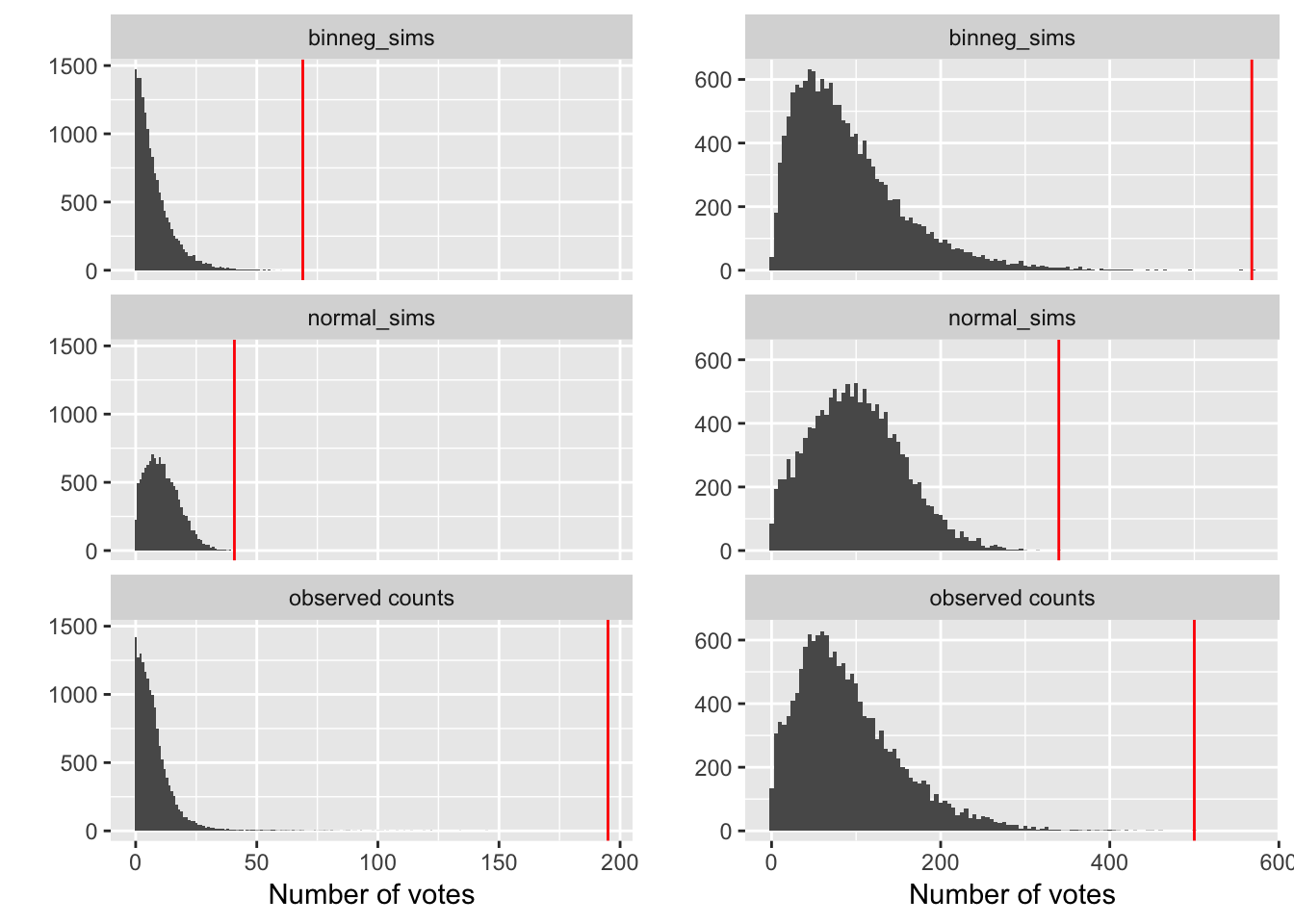
We now check a few runs with samples from the 2006 and 2012 election (warning: this code is run on parallel over 35 processes. Each data split takes about 3 minutes to run in this example):
# use same sample size as 2006 quickcount
sample_1 <- select_sample_prop(nal_2006, stratum = estrato, frac = 0.058, seed = 12)
fit_2006 <- mrp_estimation_stan(sample_1, estrato, n_iter = 700, n_warmup = 300, seed = 992,
            partidos = c("pan","pri_pvem", "panal", "prd_pt_conv", "psd", "otros"),
            frame = "nal_2006")
actual_2006 <- nal_2006 %>% select(casilla_id, pri_pvem:otros) %>%
gather(party, votes, pri_pvem:otros) %>%
group_by(party) %>% summarise(actual_votes = sum(votes)) %>%
mutate(actual = 100 * actual_votes / sum(actual_votes)) %>% select(party, actual)
fit_2006$post_summary %>% select(party, int_l, int_r) %>% left_join(actual_2006)## Joining, by = "party"## # A tibble: 7 x 4
## party int_l int_r actual
## <chr> <dbl> <dbl> <dbl>
## 1 participacion 58.1 58.6 NA
## 2 pan 35.7 36.1 35.9
## 3 prd_pt_conv 35.1 35.5 35.3
## 4 pri_pvem 22.1 22.4 22.3
## 5 otros 2.88 2.96 2.88
## 6 psd 2.67 2.73 2.70
## 7 panal 0.934 0.977 0.961sample_2 <- select_sample_prop(nal_2012, stratum = estrato, frac = 0.04, seed = 12)
fit_2012 <- mrp_estimation_stan(sample_2, estrato, n_iter = 700, n_warmup = 300, seed = 992,
partidos = c("pan", "pri_pvem", "panal", "prd_pt_mc", "otros"),
frame = "nal_2012")actual_2012 <- nal_2012 %>% select(casilla_id, pri_pvem:otros) %>%
gather(party, votes, pri_pvem:otros) %>%
group_by(party) %>% summarise(actual_votes = sum(votes)) %>%
mutate(actual = 100 * actual_votes / sum(actual_votes)) %>% select(party, actual)
fit_2012$post_summary %>% select(party, int_l, int_r) %>% left_join(actual_2012)## Joining, by = "party"## # A tibble: 6 x 4
## party int_l int_r actual
## <chr> <dbl> <dbl> <dbl>
## 1 participacion 62.9 63.4 NA
## 2 pri_pvem 38.0 38.4 38.2
## 3 prd_pt_mc 31.5 31.9 31.6
## 4 pan 25.1 25.5 25.4
## 5 otros 2.48 2.56 2.51
## 6 panal 2.24 2.31 2.29Calibration
From our point of view, the most important part of model testing was calibration performance for the interval estimates produced by our methods across past elections in Mexico, with different data perturbations that we may expect to see in incomplete samples from the election night, as it was always certain that results would have to be reported with an incomplete and probably biased sample.
Below we show the performance of three methods: traditional ratio estimates with collapsed strata when needed, a model based on a normal likelihood (NNP) with no pooling, and the negative binomial multilevel (NB-multilevel) model presented above. The numbers in the bars indicate the coverage of the intervals produced, and the length is the mean half length of the intervals produced. Colors indicate the party being estimated.
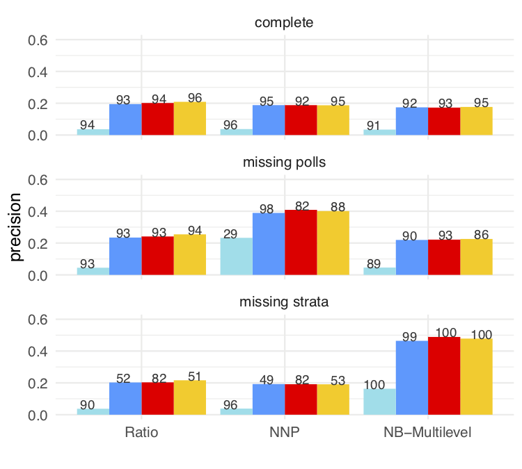
Calibration tests (100 samples)
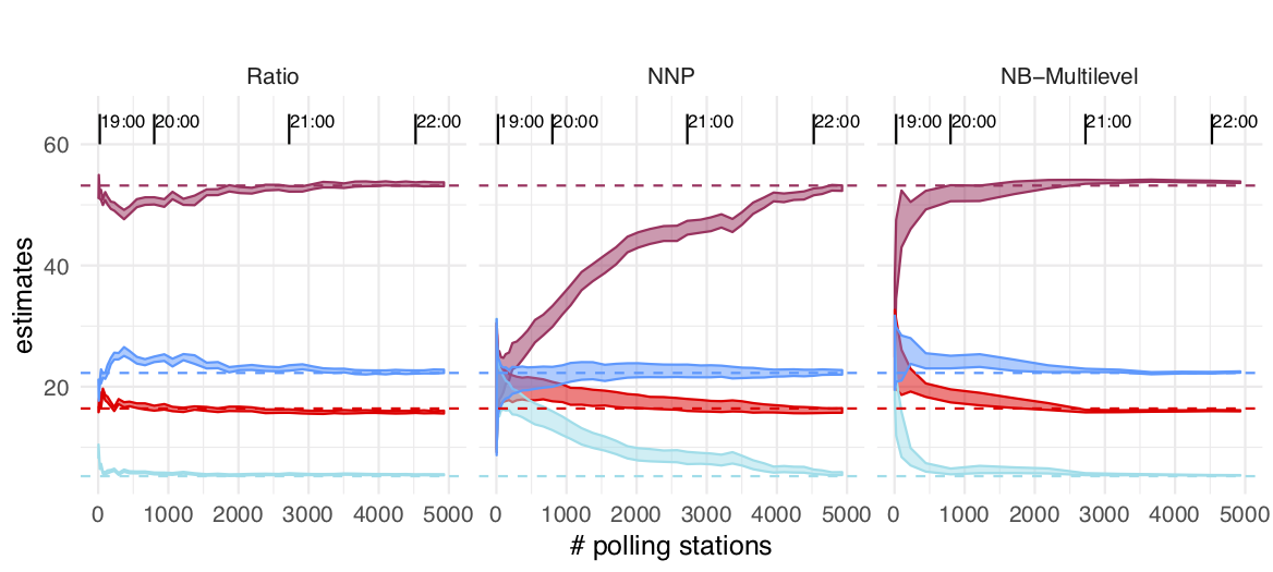
Results on the election night
We now show results for partial samples across time 2018 election night for the three methods (which were all used on that night, color indicates party):
Remesas
Additionaly we show more detailed behaviour for our model:
library(lubridate)
files_names <- list.files("data", full.names = TRUE) %>% keep(str_detect(., "anzarut"))
files_results <- map_df(files_names, ~read_csv(file = .x))
results <- files_results %>% select(-PART) %>% gather(candidate, prop, RAC:JHRC) %>%
  spread(LMU, prop) %>% rename(inf = `0`, mean=`1`,sup=`2`)
results <- results %>%
  mutate(hour = ymd_hm(paste0("2018-07-01 ",str_sub(R, 3, 4), ":", str_sub(R,5,6))))
results_filt <- results %>% filter(hour < ymd_hm("2018-07-01 21:31"))
ggplot(results_filt, aes(x=hour, y=mean, colour=candidate, group=candidate)) +
geom_line() + geom_point() +
geom_ribbon(aes(ymin = inf, ymax = sup), alpha=0.2)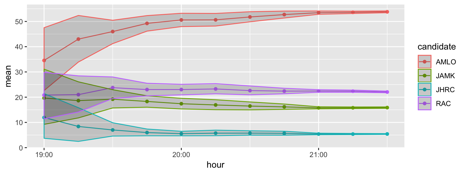
The results at 8:00 pm and 9:30 pm (at closing time of polling stations and 1:30 hours later) are
results %>% filter(hour == ymd_hm("2018-07-01 20:00"))## # A tibble: 4 x 8
## EQ EN R candidate inf mean sup hour
## <chr> <chr> <chr> <chr> <dbl> <dbl> <dbl> <dttm>
## 1 anzarut 00 012000 AMLO 48.0 50.6 53.2 2018-07-01 20:00:00
## 2 anzarut 00 012000 JAMK 15.3 17.4 19.6 2018-07-01 20:00:00
## 3 anzarut 00 012000 JHRC 4.69 5.54 6.49 2018-07-01 20:00:00
## 4 anzarut 00 012000 RAC 20.9 23.0 25.1 2018-07-01 20:00:00results %>% filter(hour == ymd_hm("2018-07-01 23:30"))## # A tibble: 4 x 8
## EQ EN R candidate inf mean sup hour
## <chr> <chr> <chr> <chr> <dbl> <dbl> <dbl> <dttm>
## 1 anzarut 00 012330 AMLO 53.3 53.5 53.8 2018-07-01 23:30:00
## 2 anzarut 00 012330 JAMK 15.8 16.0 16.2 2018-07-01 23:30:00
## 3 anzarut 00 012330 JHRC 5.2 5.29 5.37 2018-07-01 23:30:00
## 4 anzarut 00 012330 RAC 22.1 22.3 22.5 2018-07-01 23:30:00With nearly 94% of stations counted, on July 3, the actual counts are
df_prep <- data_frame(candidate = c('AMLO','RAC','JAMK','JHRC'),
           prep_94percent = round(c(52.96, 22.50, 16.40, 5.14),1))
## Warning: `data_frame()` is deprecated, use `tibble()`.
## This warning is displayed once per session.df_prep## # A tibble: 4 x 2
## candidate prep_94percent
## <chr> <dbl>
## 1 AMLO 53
## 2 RAC 22.5
## 3 JAMK 16.4
## 4 JHRC 5.1Although these results are not final, we can check that most of the cases, through all the process, the 95% intervals move smoothly, covering or nearly covered the actual preliminary counts:
res_actual <- results_filt %>% left_join(df_prep)## Joining, by = "candidate"ggplot(res_actual, aes(x=hour, y=mean, colour=candidate, group=candidate)) +
geom_ribbon(aes(ymin = inf, ymax = sup), alpha=0.2) +
geom_hline(aes(yintercept = prep_94percent, colour=candidate))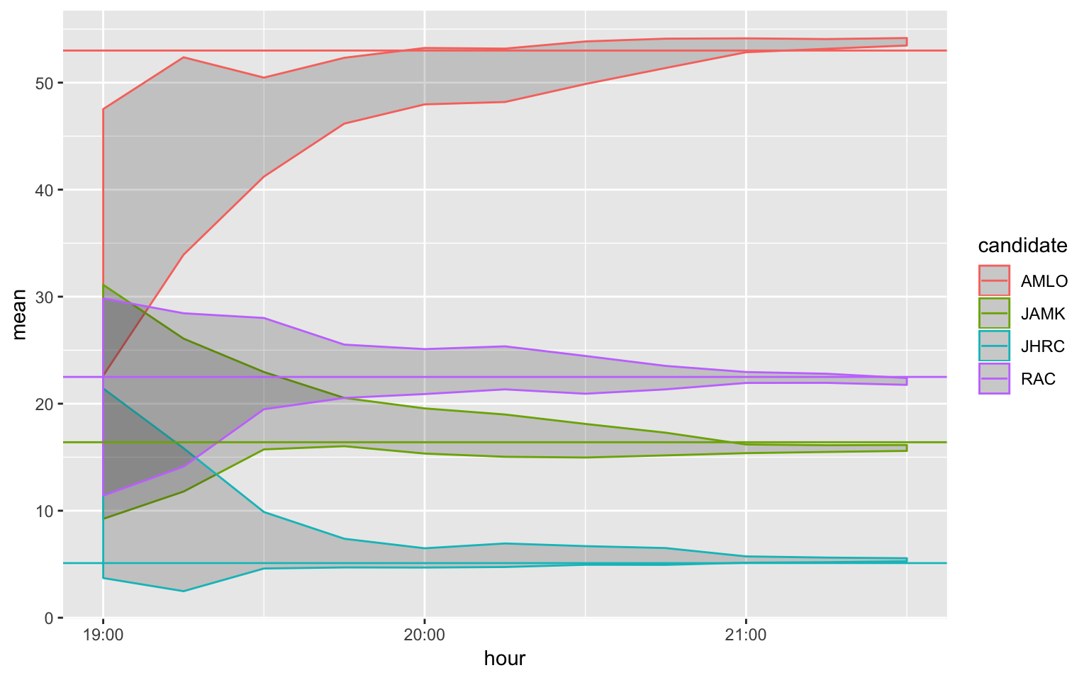
Advantages of our bayesian method fitted with Stan
- The hierarchical structure allows us to produce estimates with good coverage even in extreme situations where some strata are missing.
- In every step of the electoral process, the intervals produced by this method tend to move smoothly, with reasonable coverage even with small partial samples.
- The sensitive Stan diagnostics give early warnings of fitting problems and biased results methods.
- Data splitting allowed us to run models in less than 5-10 minutes.
Further work
- When strata are missing, the intervals produced tend to be large (close to 99% coverage), as the prior for the \(\sigma_st\) parameter is used. Further modelling of this parameter may help.
- Most methods showed evidence of slight undercoverage - the final incomplete sample reported was slightly biased, and more research is needed to understand if this could be improved by adding additional covariates, and maybe include more extreme scenarios in the calibration testing.
- Modelling of covariance between candidates may help with both efficiency and calibration, but this means further optimization efforts should be carried out to mantain run times below the needed threshold (10 minutes).
- Upper truncation of negative binomial may help also in low data situations. Our model, with little data, will tend to overestimate total vote counts. Again, this was not included for performance reasons, as truncation in the likelihood extends considerably run times for our models.
- Good convergence statistics were obtained with around 600 NUTS samples (300 warmup), although in some cases the montecarlo relative error, as reported in Stan outputs, could be relatively high (but less than 15%). Nevertheless, we consistently obtained good R-hat mixing and no divergent samples.
Gabry, Jonah, Daniel Simpson, Aki Vehtari, Michael Betancourt, and Andrew Gelman. 2017. “Visualization in Bayesian workflow.” arXiv E-Prints, September, arXiv:1709.01449.
J., Little Roderick. 2003. “The Bayesian Approach to Sample Survey Inference.” In Analysis of Survey Data, 49–57. Wiley-Blackwell. https://doi.org/10.1002/0470867205.ch4.
Park, David K., Andrew Gelman, and Joseph Bafumi. n.d. “Bayesian Multilevel Estimation with Poststratification: State-Level Estimates from National Polls.” Political Analysis 12 (4). Cambridge University Press: 375–85. https://doi.org/10.1093/pan/mph024.
Stan Development Team. 2017. Stan Modeling Language User’s Guide and Reference Manual, Version 2.17.0. http://mc-stan.org/.
———. 2018. “RStan: The R Interface to Stan.” http://mc-stan.org/.
Teresa Ortiz, Felipe González. 2018. Quickcountmx: Estimate Election Results Mexico. https://github.com/tereom/quickcountmx.